The Tachometer
Rotational speed is the most important parameter that we need to measure in the hybrid powertrain. Since all of the mechanical components are connected via the planetary gearset, knowledge of the air engine speed and electric motor speed will enable us to calculate output speed. We measure the speed of these components using a tachometer. There are many possible designs for a tachometer, but we will use one based on a 'daisy wheel' and Hall-Effect sensor.
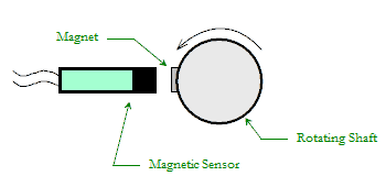
A tachometer has two main components. The first is a sensor that fires when it senses that a certain part of the rotating shaft is near. The figure at right shows a simple bicycle tachometer, which uses a magnet (usually attached to the spokes of the wheel) and a magnetic sensor. Each time the wheel rotates, the magnetic sensor sends an electrical pulse to the 'brain' of the tachometer.
We have a few choices in designing the rest of the tachometer. Probably the most obvious method would be to send the pulses directly to a digital pin on Arduino, and use its internal clock to measure the time between pulses. Taking the reciprocal of the time between pulses would give a measure of rotational speed. We have used this method at Rowan for many years, with varying degrees of success. The main problem with this approach is that it requires use of the 'interrupt' function in Arduino, which we have found (through painful experience) to be less than reliable. In short, the time spent debugging software that uses the interrupt function was found to be greater than the time spent building the tachometer itself, and the resulting tachometers were often quite noisy.
A second approach is to design a circuit that converts a pulse train into an analog voltage that is proportional to the measured speed. In other words, a fast train of pulses is converted into a high voltage, and a slow train of pulses is converted into a low voltage. This voltage is sent to an analog port on Arduino, where it is a simple matter (in software) to convert to speed in revolutions per minute. This approach is much more reliable than the first, and the resulting tachomoter is relatively noise-free. The paragraphs below describe the circuit used to construct this tachometer.
Types of sensors
The two most common types of sensor for this application are optical and Hall-Effect. The optical sensor has an LED (usually infrared) on one side of a slot, and a detector on the other side. This was the first type of sensor we tried when prototyping the tachometer, since it seemed to be the simplest (the daisywheel can be made of any opaque material). Unfortunately, we found that the optical sensor had intermittent reliability, even in a laboratory setting. What is worse, the 'faculty-prototype' seemed to work reliably, but many of the student prototypes gave spurious readings. We finally traced the problem to variations in laboratory lighting. Since the faculty prototype was always used in the same spot, there were no variations in lighting, but since the students worked wherever they could find space, the presence of sunlight wreaked havoc with the sensor. Our conclusion is that optical sensors are best suited to applications where lighting is constant and reliable, and not to a university laboratory setting.
The next most common type of interruptor sensor is Hall-Effect. In this sensor, a permanent magnet is on one side of the sensor and a detector on the other side. If the field of the magnet is altered by a ferrous material, the sensor is triggered. This requires that the daisywheel be made of steel or iron, which makes fabrication more involved than with the optical sensor. Of course, you can make the daisywheel primarily of thin plastic, and glue pieces of steel to the petals if you don't have access to a waterjet machine.
The Tachometer Circuit
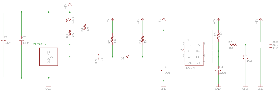
The analog tachometer circuit is shown in the schematic above. Its purpose is to measure the rotational speed of a shaft. The shaft might be the output of a motor or engine, so the usefulness of this circuit for a mechanical engineer is obvious. At first glance, the circuit probably looks confusing and overwhelming, but it can easily be divided into several modules whose function is easy to understand. We will go through each module in order, and by the end of this document you should have a good grasp on how the circuit operates.
On the simplest level, the circuit takes magnetic pulses in at one end, and generates a voltage (to be measured with Arduino) at the other end. The voltage is proportional to the speed at which the magnetic pulses arrive at the input. Thus, pulses that arrive in quick succession will generate a high voltage, and vice versa. By calibrating each voltage with its corresponding shaft speed, we can create a tachometer.
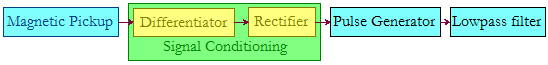
The block diagram above shows the sequence that the signal passes through the circuit. At the beginning, we have a magnetic pickup that detects the presence of a ferrous material. As one 'petal' of the daisywheel passes the pickup, its output voltage changes from low to high, then back to low again. The signal conditioning circuitry changes the pulse into a 'trigger' that is understood by the pulse generator. When the pulse generator receives a trigger, it creates a pulse of an exact duration. The lowpass filter 'calculates' the average voltage that it sees - the more pulses it sees per second, the higher the average voltage. The filter sends this averaged value to Arduino, where it can be translated into a rotational speed.
The Detector Circuit
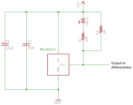
At the heart of the magnetic pickup circuit is the Melexis MLX90217 Hall Effect Geartooth Sensor. It uses the Hall effect to detect changes in magnetic flux, as when a ferrous material is nearby.
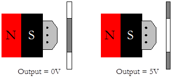
The figure at right shows a view of the sensor from the top. As you can see, a magnet has been glued to the back of the sensor, and the magnetic field passes through to the front of the sensor. It is very important that the south pole of the magnet be attached to the sensor - reversing the magnet will prevent the sensor from detecting anything. When a ferrous object (such as one of the petals of the daisywheel) is in front of the sensor, its output voltage goes to 0V (ground). When the petal moves away, the sensor outputs the power supply voltage (5V, in this case).
The LED is used as an 'idiot check', just to make sure the sensor is working. When the sensor detects the daisywheel, the lower leg of the LED goes to ground and the LED lights up. When nothing is in front of the sensor, the lower leg of the LED is at 5V. When both legs of the LED are at 5V, no current can flow and the LED remains dark.
The 300Ω resistor is used to limit the flow of current through the LED. Without it, the LED would burn out in a matter of seconds. In general, there is a 2V voltage drop across the LED. Using Ohm's law, we find that
\begin{equation} \frac{5\text{V} - 2\text{V}}{300\Omega} = 0.01\text{mA} \end{equation}flows through the LED when lit. 10mA is a nice, safe current that will light up most LEDs.
A few other, minor details: R4 is in the circuit to ensure that the output of the pickup is 5V when nothing is detected. You might think of the pickup as a switch. When it detects something ferrous, it connects the output to ground, which is 0V. When it doesn't detect anything, it disconnects the switch. With no connection between output and ground, no current flows through R4 (or the LED, either). With no current flowing through the resistor there is no voltage drop, so the lower leg of the resistor is also at 5V. This is known as a pullup resistor and is very commonly used in the output of sensors to ensure that they go 'high' when nothing is happening. Without the pullup resistor, the output would 'float'; i.e. it could take on any value between 0 and 5V.
The 10μF and 10nF capacitors are used to smooth out the power supply voltage. This way, any electromagnetic interference that is picked up by the wires leading to the tachometer won't get passed along to the signal. One really useful way to look at a capacitor is as a device that blocks low frequency signals (and DC) and passes through high frequency signals. Since EMI is high frequency, it will pass through the capacitors to ground, leaving the 5V supply line unaffected.
To summarize, the magnetic pickup circuit generates 0V when it detects the daisywheel petal, and 5V when it doesn't. The result is a regular sequence of pulses (a square wave) whose frequency depends upon the rotational speed of the daisywheel.
The Differentiator
The next few modules in the circuit transform the square wave into something that the pulse generator can recognize. First, note that the pulse generator can only be triggered by a negative pulse of very short duration. If a longer pulse is used to trigger the pulse generator, multiple output pulses may result for a single input pulse. Thus, we need a way to shorten the pulses going into the pulse generator - the shorter the better.
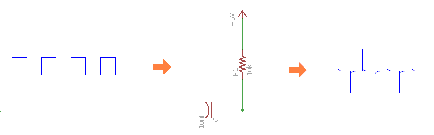
One simple way to do this is to differentiate the square wave, just like in calculus. In a square wave, the signal is steady for a while at 0V, then makes an abrupt transition to 5V where it again remains steady until it abruptly transitions back to 0V. The signal transitions from 0 to 5V in a very short time, so the derivative of the signal is essentially infinite at the transitions. Conversely, the signal remains constant between transitions, so its derivative is zero. The result of differentiating the square wave is a series of positive and negative 'spikes', as shown in the figure above.
Constructing a differentiator is surprisingly easy, as you can see by the circuit above. Recall that the capacitor allows high frequency (rapidly-changing) signals to pass through, but blocks low frequency (steady, or slowly-changing) signals. The steady parts of the square wave are blocked, while the rapid transitions are passed through as spikes. R5 serves to pull up the output when nothing is happening, in a similar manner to the pullup resistor earlier.
The Rectifier
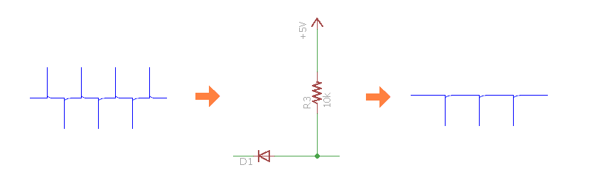
The pulse generator is triggered by negative pulses, positive pulses will confuse the pulse generator or even damage it. The purpose of the rectifier is to eliminate the positive pulses, allowing only the negative pulses to pass through. A diode (shown as D1 in the figure) allows current to pass through in only one direction. If the voltage on the left side of the diode is higher than that on the right, the resulting current will be blocked by the diode. On the other hand, if the voltage on the left side is more negative, the current will pass through unhindered (with a small voltage drop). Thus, the diode blocks positive pulses, and allows negative pulses to pass through. If we wanted only positive pulses, we would just reverse the orientation of the diode. As before, R7 acts as a pullup resistor to keep the signal at 5V when nothing is happening.
The Pulse Generator
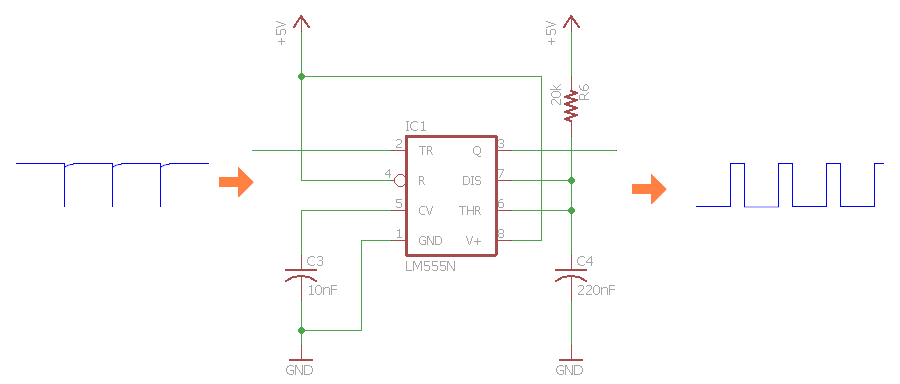
The pulse generator circuit is formed around an LM555 timer chip. The 555 is a classic chip, first introduced in 1971, that is used in everything from timers to power supplies (and tachometers!) More than 1 billion 555s are produced every year, despite the age of the design.
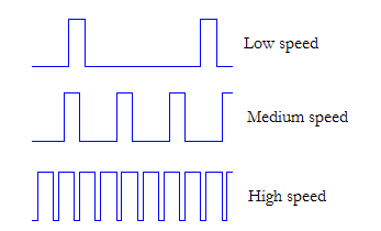
The 555 in the circuit above is configured as a 'one-shot'. That is, it sends out a pulse of a precise duration every time it receives a trigger signal. Once the pulse has been generated, the 555 does nothing until it gets another trigger input. Thus, every time the 555 receives a trigger input, it generates a pulse with a specified width. The square wave generated by the 555 timer is directly related to the number of daisy wheel 'petals' the Hall-effect sensor detects. At right are sample pulse trains generated by the 555 timer at different speeds.
According to the datasheet, the 555 can generate pulses anywhere from microseconds to hours in duration! The duration of the pulse is determined by the values of R6 and C4 according to the following equation
\begin{equation} T=1.1R_{6}C_{4} \end{equation}So now we must do a little math to determine the desired length for the pulses coming out of the pulse generator for our daisy wheel setup and expected speed range. Let the number of slots in the daisywheel be Ns, and the speed of the rotating shaft be n. Then the time between pulses from the daisywheel is
\begin{equation} T=\frac{60}{nN_{s}} \end{equation}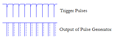
where the 60 is used to convert from revolutions per minute to revolutions per second. For example, if the shaft is rotating at 2000rpm and there are 6 slots in the daisywheel, then the time between pulses is 5ms. If we were to incorrectly choose R6 and C4, such that the 555 timer produced a pulse width of 6ms, then more pulses would be received by the 555 timer than it could produce. This means pulses from the generator will 'overlap' each other and the output will remain at a constant 5V, as shown in the figure at right. Further increases in speed will not change the output, and so our tachometer is useless at these high speeds.
Our goal, then, is to make the pulses from the pulse generator just wide enough to begin to overlap at the maximum expected speed. You might wonder why we don't just make the pulses really narrow, so as to have an almost unlimited maximum speed. Recall that the next circuit in the chain will take the average value of the output of the 555. If the pulses remain narrow regardless of speed, the output voltage will stay very low and it will be tough for Arduino to make distinctions between speeds. For the best resolution, we'd like the maximum expected speed to correspond to 5V at the output, with the minimum speed being somewhere around 0V. Thus, the pulses coming out of the 555 should be approximately equal to the time between pulses from the daisywheel at maximum speed.
It is much easier to keep the capacitor value constant (since there is a much smaller variety of capacitor values) and change the resistor to achieve the desired pulse length. The equation for the proper resistor value (assuming that the output pulse and daisywheel pulse are set equal) is
\begin{equation} \frac{60}{nN_{s}}=T=1.1R_{6}C_{4} \end{equation} \begin{equation} R_{6}=\frac{60}{1.1nN_{s}C_{4}} \end{equation}Thus, for 2000rpm and 6 slots, the correct resistor value is 20,661Ω. Of course, you won't find a resistor with exactly that value, but 20k is close enough. In our circuit, the pulse length is
\begin{equation} T=1.1\cdot 20\text{k}\Omega \cdot 220\text{nF}=4.84\text{ms} \end{equation}We would not want to round up to 22kΩ (the next available resistor), since it will produce a 555 timer pulse length of 5.32ms, which will cause the tachometer to saturate below 2,000rpm.
\begin{equation} T=1.1\cdot 22\text{k}\Omega \cdot 220\text{nF}=5.32\text{ms} \end{equation}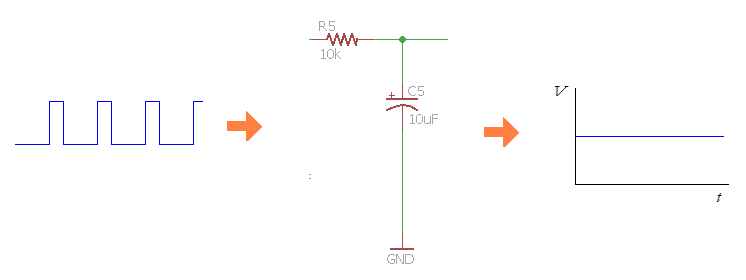
The Lowpass Filter
The final stage in the circuit is the lowpass filter. The lowpass filter removes any high frequency content from the signal (the pulses) and passes along low frequency (and DC) signals. For our circuit, the lowpass filter passes along the average value of the voltage coming into it. If the pulses are close together, the average voltage is high, and if the pulses are widely spaced, the average value is low. The lowpass filter has a cutoff frequency given by
\begin{equation} f_{c}=\frac{1}{2\pi R_{5}C_{5}}=1.59\text{Hz} \end{equation}This means that the filter blocks anything above 1.59Hz, and allows anything below 1.59Hz to pass through. As with everything electronic, this circuit design is a tradeoff. If we make the cutoff frequency very low, it will make the output signal nice and smooth, but will be very sluggish in responding to changes in speed. If we make it very high, much of the choppy nature of the pulses will be passed through, and it will be hard for Arduino to measure the speed correctly. The 1.59Hz represents a tradeoff between smoothness and response time.
You may notice that the output is still a little choppy at very low speeds (less than 100rpm). One remedy for this is to add a second, identical lowpass filter right after the first, which makes it a second-order lowpass filter. Another option is to use a moving-average filter in the Arduino code to smooth out the pulses. In the printed circuit board (described below) we use only a first-order filter.
The Printed Circuit Board
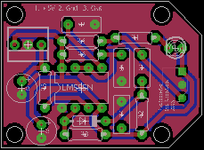
To make your own tachometer, you can fabricate the circuit described above on a perfboard, or you can use the Eagle CAD files listed here to have a printed circuit board made. Right-click on each file and select 'Save link as' to download the files, otherwise your browser might try to interpret the XML-format files.
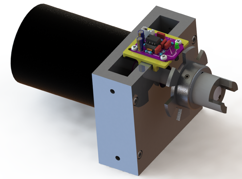
The board is laid out such that the components are soldered on to the top side and the Hall-effect sensor (with its magnet glued on) is soldered to the bottom side. A 3-pin connector with 0.1 inch spacing is used to hook the board up to Arduino. The figure below shows a rendering of the tachometer circuit board mounted to a DC motor with daisy wheel. Note that the PCB is purple - OSH Park is my favorite PCB maker, and they're even based in Oregon!